
Solving simple optimization problems with Groovy® using Commons Math, Hipparchus, OptaPlanner, and Timefold
Published: 2024-03-14 10:22PM (Last updated: 2026-09-05 08:00AM)
Introduction
There are many problems involving optimization. We’ll explore a case study which can be solved using linear optimization, also known as linear programming. Linear programming problems optimize a particular linear objective function subject to one or more linear equality and inequality constraints.
We’ll look at such a problem and some libraries and tools which can be used to solve them.
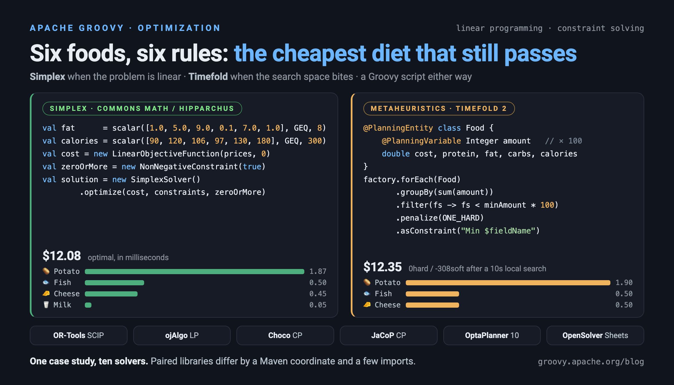
Case Study: Diet Optimization
Let’s look at a case study where we try to minimize the cost of food items in our diet, while still maintaining some overall constraints which we might set for health or dietary preference reasons. The example is inspired by this SAS example, but see the Further Information section for a more elaborate linear programming example, the classic Stigler diet problem, solved using Google OR-Tools.
First, here are six foods with their costs and nutritional values that make up our diet:
Bread 🍞 |
Milk 🥛 |
Cheese 🧀 |
Potato 🥔 |
Fish 🐟 |
Yogurt 🍶 |
|
Cost |
2.0 |
3.5 |
8.0 |
1.5 |
11.0 |
1.0 |
Protein (g) |
4.0 |
8.0 |
7.0 |
1.3 |
8.0 |
9.2 |
Fat (g) |
1.0 |
5.0 |
9.0 |
0.1 |
7.0 |
1.0 |
Carbohydrates (g) |
15.0 |
11.7 |
0.4 |
22.6 |
0.0 |
17.0 |
Calories |
90 |
120 |
106 |
97 |
130 |
180 |
We want to minimize cost, while maintaining optimal nutrition, where optimal will be defined as meeting the following criteria:
-
Must be at least 300 calories
-
Not more than 10 grams of fat
-
Not less than 10 grams of carbohydrates
-
Not less than 8 grams of fat
-
At least 0.5 units of fish
-
No more than 1 unit of milk
Note, we don’t recommend this simplified set of constraints as a real diet, it is only for illustrative purposes for our case study.
Relating this back to our earlier definition of linear programming, our list above represent our linear constraints. Our object function is cost which is determined by the amount of each food multiplied by its cost.
Solving with a spreadsheet solver
This kind of problem is so common that solvers exist even within spreadsheet applications. We’ll show a solution using the OpenSolver Add-on for Google Sheets. But you can do the same thing using Microsoft Excel if you prefer.
First, we fill in the data for our problem. It will be similar to the figure shown below, but initially, the variable cells (blue) and objective cell (yellow) will be blank.
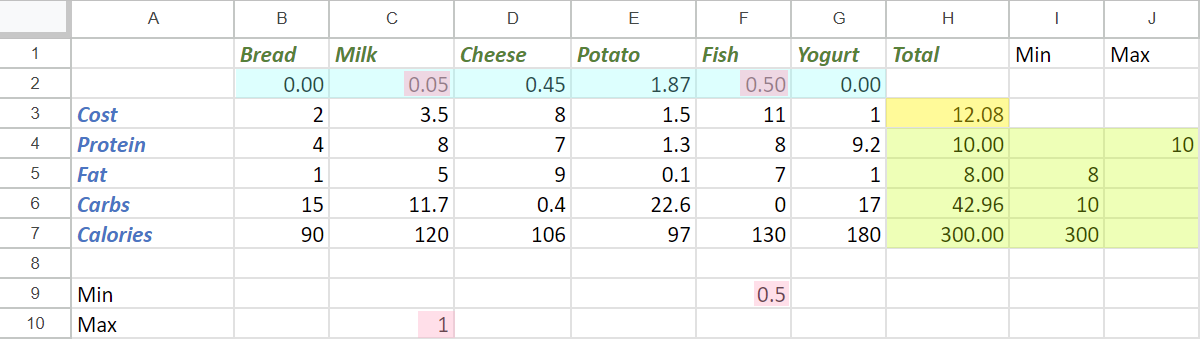
Then, using the OpenSolver extension, we identify by way of cell ranges, our data (blue) and objective (yellow) cells, as well as the constraints.
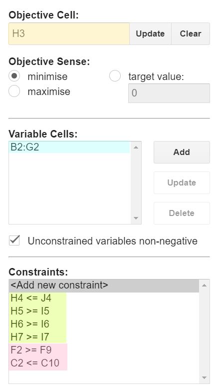
Then we click "Solve" and it calculates our optimized value.
Let’s look at solving this programmatically using Groovy. Groovy provides a particularly nice environment for scripting solutions to such problems, but for the libraries we are using, it should be possible to use most JVM languages.
Using Apache Commons Math or Hipparchus
Let’s now look at solving this problem using a simplex solver.
We’ll use the SimplexSolver class from Apache Commons
Math which is essentially the same as the one from Hipparchus
(a commons math fork).
We’ll start with a little helper method for defining our constraints:
static scalar(coeffs, rel, double value) {
    new LinearConstraint(coeffs as double[], rel, value)
}
Next we define our individual constraints and the combined set:
val milk_max   = scalar([0, 1, 0, 0, 0, 0], LEQ, 1)
val fish_min   = scalar([0, 0, 0, 0, 1, 0], GEQ, 0.5)
val protein    = scalar([4.0, 8.0, 7.0, 1.3, 8.0, 9.2],     LEQ, 10)
val fat        = scalar([1.0, 5.0, 9.0, 0.1, 7.0, 1.0],     GEQ, 8)
val carbs      = scalar([15.0, 11.7, 0.4, 22.6, 0.0, 17.0], GEQ, 10)
val calories   = scalar([90, 120, 106, 97, 130, 180],       GEQ, 300)

LinearConstraintSet constraints = [milk_max, fish_min, protein, fat, carbs, calories]
Each individual constraint has a coefficient for each food,
a relationship, and a value.
We’re using Groovy 6’s val keyword for these declarations.
It is the immutable companion to var; on earlier Groovy versions,
var or def work just as well.
Next, we define our cost function, and an additional constraint
to indicate that we can’t buy a negative amount of any food.
The zeroOrMore constraint saves us from doing the long-hand
equivalent, like fish_min but with a minimum of 0, for each food.
val cost = new LinearObjectiveFunction([2.0, 3.5, 8.0, 1.5, 11.0, 1.0] as double[], 0)

val zeroOrMore = new NonNegativeConstraint(true)
Now, our solution is found by creating a new solver, and asking
it to optimize using our cost function and the constraints.
We then print our solution out, one line per food that made the cut.
The bar helper is a small addition in Groovy 5 which renders a value
as an ascii bar; here the bars are scaled so that 2 units fill the width:
import static org.codehaus.groovy.util.StringUtil.bar

val solution = new SimplexSolver().optimize(cost, constraints, zeroOrMore)

static pretty(int idx, BigDecimal d) {
    d ? [sprintf('%s %s %.2f', ['🍞', '🥛', '🧀', '🥔', '🐟', '🍶'][idx], bar(d, 0, 2, 20), d)] : []
}

if (solution != null) {
    printf "Cost: %.2f%n", solution.value
    println solution.point.indexed().collectMany(this::pretty).join('\n')
}
When run, it gives the following output:
Cost: 12.08
🥛 ▋ 0.05
🧀 ████▌ 0.45
🥔 ██████████████████▊ 1.87
🐟 █████▏ 0.50
This is the same solution as what we saw when using the spreadsheet.
You can currently swap between Apache Commons Math and Hipparchus by switching the Maven coordinates of the jar being used on the classpath and changing a few import statements. This may change in future versions, but for now:
-
Using
org.apache.commons:commons-math3:3.6.1gives an older stable version of Commons Math, now a decade old. -
Using
org.apache.commons:commons-math4-legacy:4.0-beta1gives the latest version of these classes from Apache Commons Math. The naming possibly deserves some explanation. There has been ongoing effort to modularise Commons Math and there are numerous components delivered as a result. The optimisation classes haven’t been worked on yet and are available in the aforementioned artifact, which hasn’t seen a new release since late 2022. -
Using
org.hipparchus:hipparchus-optim:4.0.3gives classes from the forked project. For the classes we are using, there is essentially no difference in the fork, but other parts of the library have seen useful updates if you don’t mind having a dependency that isn’t backed by the ASF.
If you don’t like those options, there are many more, here are a few with Groovy solutions in the same repo as the above examples:
-
For a solution using the SCIP simplex solver in Google OR-Tools, see DietOrTools.groovy
-
For a solution showing Groovy support within SAS, see DietGroovy.sas
-
For a solution using the LP solver in ojAlgo, see DietOjalgo.groovy
-
For a solution using the Choco constraint programming solver, see DietChocoInt.groovy for a solution using scaled integers, and DietChocoReal.groovy for a solution with real numbers using Ibex integration
-
For a solution using the JaCoP constraint programming solver, see DietJacopInt.groovy for a solution using scaled integers, and DietJacopIntKnapsack.groovy for a solution utilizing a Knapsack constraint
For simple optimization problems, like our case study, which can be solved using a simplex solver, you generally need look no further. It is a very efficient approach to solving such problems. For an additional class of slightly more complex problems, they can be mapped to linear programming problems with a little ingenuity.
For more complex problems, there are generally no super efficient solution approaches. You need to bring to bear a range of techniques for managing the potentially huge search space which is inherent in such problems. That is where optimization libraries like OptaPlanner (and Timefold) come into play.
Using OptaPlanner or Timefold
OptaPlanner is an optimization library combining optimization algorithms with constraint solving. For about a decade the library was developed under Red Hat’s guidance. In 2023, the project and other related projects were donated to the ASF as part of Apache KIE (incubating). The library was also forked as Timefold.
The two projects have since drifted apart. OptaPlanner continues under Apache KIE, with version 10 being current at the time of writing. Timefold Solver 2.0 (April 2026) was its first major release since the fork: it removed the previously deprecated APIs, so it is no longer source-compatible with OptaPlanner, and it requires JDK 21 or later. Some score-analysis and explainability features also moved to Timefold’s commercial edition, though nothing we use here.
In this blog, we’ll use Timefold. The OptaPlanner version of the same example lives alongside it in the referenced repository and is nearly identical: apart from the Maven coordinate and imports, a handful of API details differ, which we’ll point out as we go.
One of the claims of the Timefold project is that it has a lighter dependency footprint.
This can be confirmed by running the printRuntimeClasspath task in the associated builds.
Timefold has 22 dependent jars compared with OptaPlanner’s 57 jars.
While Timefold’s power isn’t needed for our simple problem, let’s examine how you would use it for the same case study.
First, we’ll create a planning entity. This is a class which the solver knows will change over time and will contain one or more planning variables.
In our case, we have just one planning variable,
the amount property, which the solver will adjust while trying
to find an optimal solution.
@PlanningEntity
@TupleConstructor(includeFields = true)
class Food {
    final String name, emoji
    final double cost, protein, fat, carbs, calories
    @PlanningVariable(valueRangeProviderRefs = "amount")
    Integer amount // times 100
}
We are using an Integer as the type for amount, since
Integers are much easier for a solver to work with.
We’ll actually store the amount (as seen in the earlier example)
multiplied by 100, but we’ll divide by 100 when displaying the result.
The other fields of our class are constants once defined during instance construction.
Next, we define a planning solution class. This has all the
information needed about any given solution including a score.
The score lets us determine whether one solution is more optimal
than another, and also whether a given solution meets all hard
and soft constraints (explained shortly).
@PlanningSolution
class DietSolution {
    @PlanningEntityCollectionProperty
    List<Food> foods

    @ValueRangeProvider(id = "amount")
    ValueRange<Integer> getAmount() {
        ValueRangeFactory.createIntValueRange(0, 200, 5)
    }

    @PlanningScore
    HardSoftScore score

    String toString() {
        val sb = new StringBuilder()
        for (f in foods) {
            sb << "$f.emoji $f.name: ${f.amount / 100}\n"
        }
        for (name in ['fat', 'carbs', 'protein', 'calories', 'cost']) {
            val total = foods.sum{ f -> f."$name" * f.amount / 100 }
            sb << sprintf("Total %s: %.2f%n", name, total)
        }
        sb << "Score: $score"
        sb
    }
}
The value range gives the solver the allowed amounts: 0 to 200 in steps of 5.
Timefold 2 simplified its value range API to a single ValueRange type;
OptaPlanner (and Timefold 1.x) call this CountableValueRange.
Next we want to define some constraints. In general, we have hard constraints which must be met and soft constraints which should be met if possible. In our case, we’ll have constraints like minimum and maximum values for various foods and various nutritional measures.
class DietConstraintProvider implements ConstraintProvider {
    @Override
    Constraint[] defineConstraints(ConstraintFactory factory) {
        new Constraint[]{
                maxField(factory, 'protein', 10),
                minField(factory, 'fat', 8),
                minField(factory, 'carbs', 10),
                minField(factory, 'calories', 300),
                minFood(factory, 'Fish', 50),
                maxFood(factory, 'Milk', 100),
                minCost(factory),
        }
    }

    private static long amountOf(Food f, String name) {
        (f."$name" * f.amount).toLong()
    }

    private static Constraint minField(ConstraintFactory factory, String fieldName, double minAmount) {
        ToLongFunction<Food> amount = f -> amountOf(f, fieldName)
        factory.forEach(Food)
                .groupBy(sum(amount))
                .filter(fs -> fs < minAmount * 100)
                .penalize(ONE_HARD)
                .asConstraint("Min $fieldName")
    }

    private static Constraint maxField(ConstraintFactory factory, String fieldName, double maxAmount) {
        ToLongFunction<Food> amount = f -> amountOf(f, fieldName)
        factory.forEach(Food)
                .groupBy(sum(amount))
                .filter(fs -> fs > maxAmount * 100)
                .penalize(ONE_HARD)
                .asConstraint("Max $fieldName")
    }

    private static Constraint minFood(ConstraintFactory factory, String foodName, double minAmount) {
        factory.forEach(Food)
                .filter(f -> f.name == foodName && f.amount < minAmount)
                .penalize(ONE_HARD)
                .asConstraint("Min $foodName")
    }

    private static Constraint maxFood(ConstraintFactory factory, String foodName, double maxAmount) {
        factory.forEach(Food)
                .filter(f -> f.name == foodName && f.amount > maxAmount)
                .penalize(ONE_HARD)
                .asConstraint("Max $foodName")
    }

    private static ToLongFunction<Food> totalCost = f ->
        (f.cost * f.amount).toLong()

    private static Constraint minCost(ConstraintFactory factory) {
        factory.forEach(Food)
                .filter(f -> f.amount > 0)
                .groupBy(sum(totalCost))
                .penalize(ONE_SOFT, fs -> fs >> 2)
                .asConstraint('Min cost')
    }
}
The sum collector groups the foods and adds up a per-food amount.
Timefold 2 dropped the int variants of its collectors, so the amounts
are supplied as ToLongFunction`s; the OptaPlanner version uses `ToIntFunction.
With these helper classes in place, we are now ready to define our problem and solve it:
import module ai.timefold.solver.core

val unsolved = new DietSolution(foods: [
        new Food('Bread' , '🍞',  2.0, 4.0, 1.0, 15.0,  90),
        new Food('Milk'  , '🥛',  3.5, 8.0, 5.0, 11.7, 120),
        new Food('Cheese', '🧀',  8.0, 7.0, 9.0,  0.4, 106),
        new Food('Potato', '🥔',  1.5, 1.3, 0.1, 22.6,  97),
        new Food('Fish'  , '🐟', 11.0, 8.0, 7.0,  0.0, 130),
        new Food('Yogurt', '🍶',  1.0, 9.2, 1.0, 17.0, 180)
])

val config = new SolverConfig()
        .withSolutionClass(DietSolution)
        .withEntityClasses(Food)
        .withConstraintProviderClass(DietConstraintProvider)
        .withTerminationSpentLimit(Duration.ofSeconds(10))

val factory = SolverFactory.create(config)
val solver = factory.buildSolver()
println solver.solve(unsolved)
Timefold 2 ships as a proper Java module, so the import module line,
a Groovy 6 feature mirroring Java’s JEP 511, replaces the half-dozen imports
we would otherwise need for the solver, its configuration classes and the
algorithm enums. (Duration needs no import at all since Groovy 5
auto-imports java.time.)
It has this output when run:
07:29:52.936 [main] INFO  a.t.s.core.impl.solver.DefaultSolver - Solving started: time spent (2), best score (0hard/0soft), environment mode (PHASE_ASSERT), move thread count (NONE), random (seed 0).
07:29:52.938 [main] INFO  a.t.s.core.impl.solver.DefaultSolver - Problem scale: genuine entity count (6), genuine variable count (6), approximate value count (40), approximate problem scale (4,096,000,000).
07:29:52.998 [main] INFO  a.t.s.c.i.c.DefaultConstructionHeuristicPhase - Construction Heuristic phase (0) ended: time spent (64), best score (-1hard/-521soft), move evaluation speed (4067/sec), step total (6).
07:30:02.935 [main] INFO  a.t.s.c.i.l.DefaultLocalSearchPhase - Local Search phase (1) ended: time spent (10001), best score (-1hard/-281soft), move evaluation speed (419407/sec), step total (613).
07:30:02.936 [main] INFO  a.t.s.core.impl.solver.DefaultSolver - Solving ended: time spent (10001), best score (-1hard/-281soft), move evaluation speed (416747/sec), phase total (2), environment mode (PHASE_ASSERT), move thread count (NONE).
🍞 Bread: 0.45
🥛 Milk: 0.8
🧀 Cheese: 0.1
🥔 Potato: 0.65
🐟 Fish: 0.5
🍶 Yogurt: 0.3
Total fat: 9.22
Total carbs: 35.94
Total protein: 16.51
Total calories: 329.15
Total cost: 11.28
Score: -1hard/-281soft
Given the amount of time we gave the solver, and using the default search algorithms, we couldn’t even meet all hard constraints. The search space was so vast, that we never reached an area in the search space where all constraints were met.
The good news is that we can provide additional guidance, so that
the solver heads in better directions during its searching.
Here is one possible additional configuration that we could supply,
along with the updated config definition:
val construction = new ConstructionHeuristicPhaseConfig(
        constructionHeuristicType: FIRST_FIT)
val moveSelector = new UnionMoveSelectorConfig([
        new ChangeMoveSelectorConfig(),
        new SwapMoveSelectorConfig()
])
val localSearch = new LocalSearchPhaseConfig(
        localSearchType: VARIABLE_NEIGHBORHOOD_DESCENT,
        moveSelectorConfig: moveSelector)
val config = new SolverConfig()
        .withSolutionClass(DietSolution)
        .withEntityClasses(Food)
        .withConstraintProviderClass(DietConstraintProvider)
        .withPhases(construction, localSearch) // additional solution guidance
        .withTerminationSpentLimit(Duration.ofSeconds(10))
It now has this output when run (log lines omitted):
🍞 Bread: 0
🥛 Milk: 0
🧀 Cheese: 0.5
🥔 Potato: 1.9
🐟 Fish: 0.5
🍶 Yogurt: 0
Total fat: 8.19
Total carbs: 43.14
Total protein: 9.97
Total calories: 302.30
Total cost: 12.35
Score: 0hard/-308soft
We can see here that it is now close to what linear programming would give us.
Further Information
-
OR-Tools linear optimization
-
A related but more elaborate example based on the Stigler Diet problem using Google OR-Tools
-
A Python Diet example also using Google OR-Tools
-
GitHub repos containing sample code:
Diet DietOptaPlanner DietTimefold
Conclusion
We have looked at using Groovy and a few linear optimization libraries to solve a diet case study. Our main focus was the Apache Commons Math and Hipparchus libraries. We also explored using the more powerful Timefold and OptaPlanner libraries.